
Overview
The HLS harmonization process takes advantage of the similarity in spectral bandpasses, spatial resolutions, and overpass time between Landsat 8/9 and Sentinel-2 A/B/C satellites to make observations comparable as if they had come from the same sensor.
By the term “harmonized,” we mean that the HLS products are results of:
- Atmospheric correction to surface reflectance;
- Cloud and cloud shadow masking;
- Normalization to a nadir-view geometry via Bi-directional Reflectance Distribution Function (BRDF) estimation;
- Spectral bandpass adjustment of one group of sensors with the other group as reference for internal data consistency;
- Gridding to a common pixel resolution, projection, and spatial extent (i.e., tile);
- Presentation of spectral data and metadata in standard format.
The harmonization algorithms are described in detail below and in the HLS v2.0 User Guide.
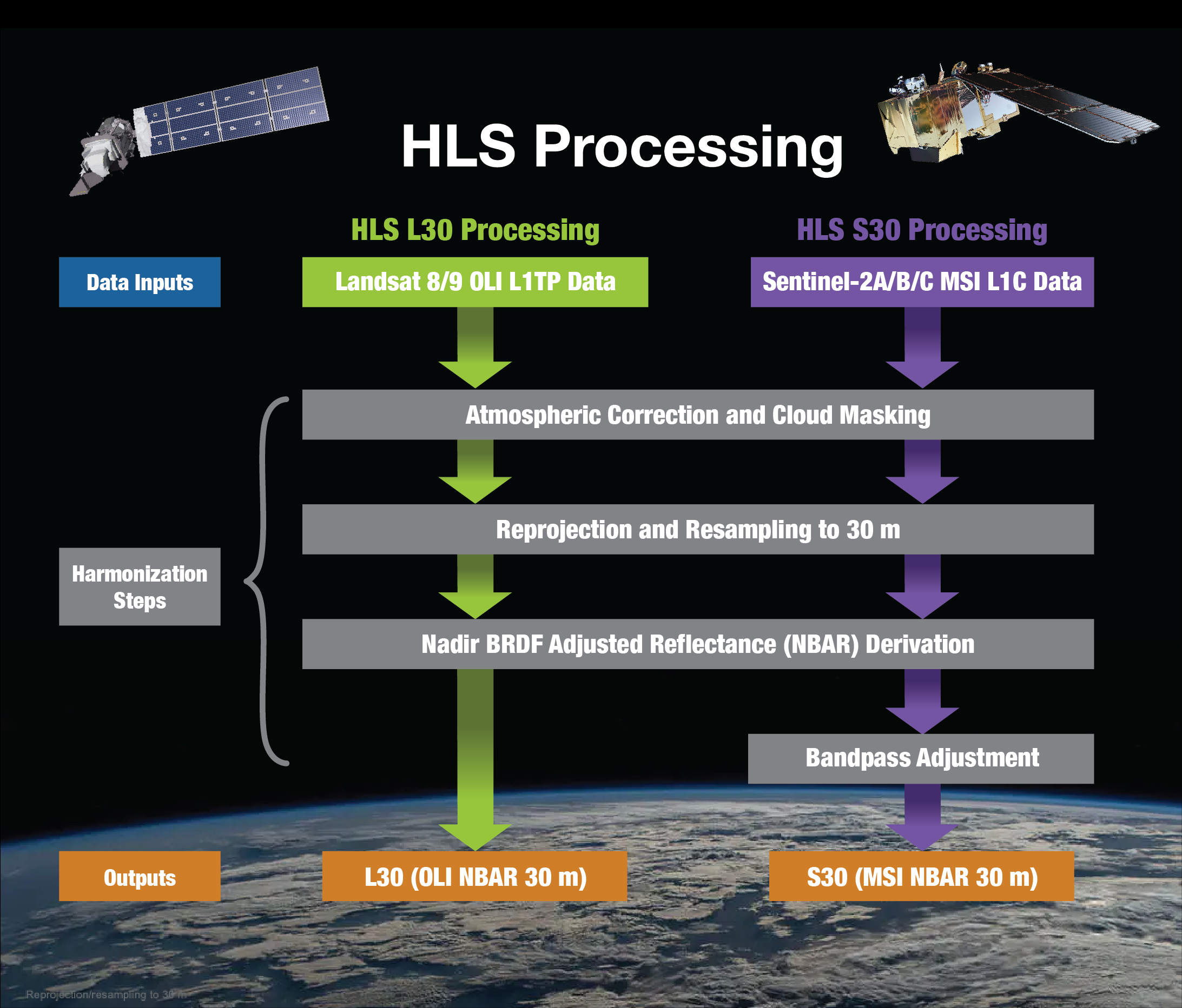
Overview of the methods applied for processing and harmonizing Landsat 8/9 and Sentinel-2 data.
Atmospheric Correction
The surface reflectance derivation from Landsat and Sentinel-2 images uses Land Surface Reflectance Code (LaSRC) originally developed by Eric Vermote (NASA/GSFC)1,2 and adapted by USGS Earth Resources Observation and Science (EROS) Center for operational use. The LaSRC performance has been evaluated in Doxani et al., 2018, 2023.3,4 A detailed description of the operational Landsat surface reflectance and its ancillary layers are provided by the U.S. Geological Survey.
LaSRC derives surface reflectance with the aerosol optical thickness retrieved from the images assuming a continental aerosol model and using ancillary data from multiple sources. The ancillary atmospheric ozone and water vapor data for gaseous absorption correction are from the MODIS 0.05° Climate Modeling Grid (CMG) data (before May 2024) or from VIIRS 0.05° CMG (after May 2024). Standard sea level atmospheric pressure is adjusted for 0.05° resolution local elevation in molecular (Rayleigh) scattering correction. The aerosol optical thickness retrieval uses the spatially explicit ratios of the red to blue surface reflectances, also in the 0.05° CMG grid, that are characterized from 10-year MODIS observations; the spectral ratio data are adjusted by the observed finer-resolution Landsat and Sentinel-2 data in spectral bands less sensitive to the aerosol effects.1,2 The HLS L30 product also includes the two thermal-infrared bands from the Landsat 8/9 TIRS sensor. The data values for these bands are not atmospherically corrected, i.e., are brightness temperature.
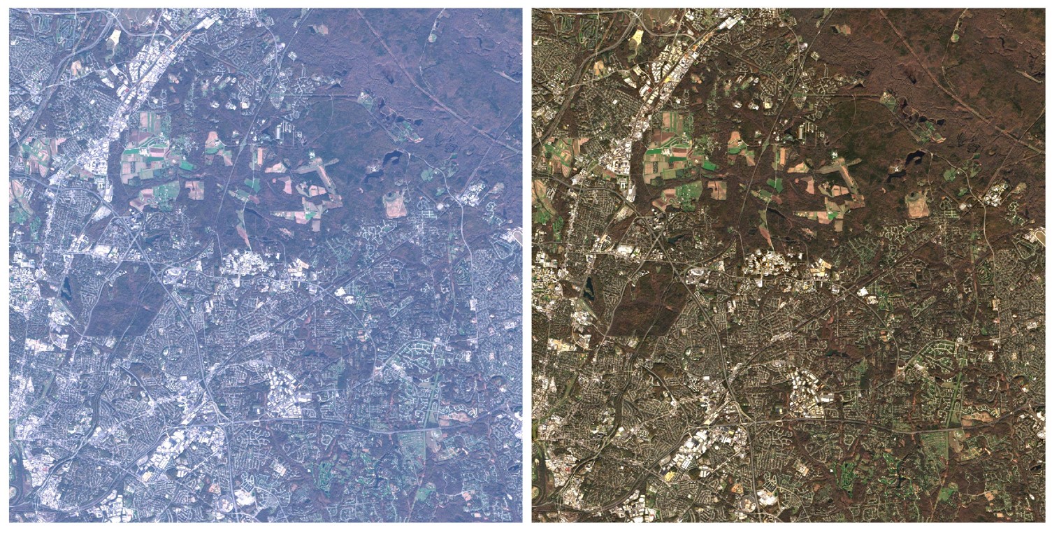
A true color composite (bands 4-3-2) of a Sentinel-2B image with top-of-atmosphere (TOA) reflectance (left) and LaSRC atmospherically-corrected surface reflectance (right). The same contrast stretch was applied to both images. Acquired on November 17, 2017 over NASA GSFC and surrounding areas (tile 18SUJ).
Cloud Masking and Quality Assessment
HLS provides per-pixel mask of cloud, cloud shadow, snow, water, and aerosol optical thickness levels. In earlier versions of HLS, the cloud and shadow masks were a union of results from multiple sources, but in HLS v2.0, they were generated exclusively by Fmask version 4.7,5,6 an update of previous Fmask versions.7,8 Fmask was found to be one of the better performing algorithms when assessed on a variety of test data sites.9,10 The Fmask cloud and cloud shadow output is dilated by 150 m during HLS processing and the dilated area is labeled as “adjacent to cloud/shadow.” The data user can treat the dilated area as clear if data loss is a concern. The mask labels and the dilation (cloud, shadow, snow/ice, water, adjacency) are stored in bits 1-5 in the per-pixel quality assessment (QA) band. The QA band also records, in bits 6 and 7, the aerosol optical thickness level (low, medium, or high) derived during atmospheric correction. The QA band is named after the cloud masking algorithm Fmask, but contains both Fmask output and the LaSRC aerosol optical thickness level information. The use of pixels with high aerosol optical thickness is not recommended.
Spatial Co-registration
HLS has adopted the Universal Transverse Mercator (UTM)-based Military Grid Reference System (MGRS) into which ESA grids the Sentinel-2 Level-1C (L1C) data. Although the USGS Landsat data are also in UTM projection and the HLS output pixel size is 30 m, the input 30-m Landsat data can not be simply copied over because the UTM coordinate origin for Landsat corresponds to the center of a 30-m pixel, while in the MGRS system it corresponds to a pixel corner. That is, even when the input Landsat data and an MGRS tile are in the same UTM zone, there is a 15-m shift between the reference points. The HLS resampling of Landsat spectral data uses the cubic convolution method. If the input Landsat scene and the MGRS tile are in two adjacent UTM zones, reprojection of Landsat is needed before resampling. The resampling of the accompanying categorical QA values only considers the inner 2 x 2 pixels in the cubic convolution kernel, and the presence of any label there will turn on the corresponding output QA bit. Because the 2 x 2 pixels may have different cloud mask labels, an output HLS pixel may have multiple bits set to 1 in its QA byte; for the aerosol optical thickness level, the label of the highest aerosol level in the inner 4 pixels is chosen for output.
The 10-m, 20-m Sentinel-2 spectral data are resampled to 30 m with an area-weighted average, and pixels in the 60-m bands are evenly split into four 30-m pixels. The cloud mask labels (derived at 20 m) and the categorical LaSRC aerosol thickness levels (derived at 10 m) are resampled to 30 m from the overlapping input pixels with a rule similar to the Landsat categorical data resampling.
BRDF Normalization
Landsat OLI and Sentinel-2 MSI are narrow field-of-view sensors, but the view angle effect is still noticeable in the contrasting backward and forward view image pairs acquired on the same day or a few days apart. HLS processing normalizes this view angle effect by predicting a nadir-view reflectance with a Bidirectional Reflectance Distribution Function (BRDF)-based c-factor technique.11,12 The end result is 30-m Nadir BRDF-Adjusted Reflectance (NBAR) – for Landsat-derived HLS this is the final L30 product, whereas Sentinel-2 NBAR undergoes a subsequent bandpass adjustment to produce the final S30 product.
The HLS BRDF normalization uses a set of constant BRDF coefficients, derived from 12-month MODIS 500-m global BRDF product.13,14,15 The derived BRDF coefficients are applied to OLI and MSI bands equivalent to MODIS ones. For the normalization of the Sentinel-2 MSI red-edge bands (705, 740, and 783 nm) that have no MODIS equivalents, the linearly interpolated BRDF coefficients from the enclosing MODIS red and NIR wavelength bands are used.12 The technique has been evaluated using off-nadir (i.e. in the overlap areas of adjacent swaths) ETM+ data11 and MSI data.16 The BRDF coefficients for the three kernels (isotropic fiso, geometric fgeo, and volumetric fvol) of the Ross–Li semiempirical model are shown in Table 1. The kernel definitions are described in the ATBD of the MOD43A1 product17 and the operational implementation for MODIS BRDF/albedo product are described in Schaaf et al., 2002.13
Table 1: BRDF coefficients used in the HLS V2.0 c-factor normalization.11,12,18
| Band name | HLS L30 Band Code | HLS S30 Band Code | Equivalent MODIS band | fiso | fgeo | fvol |
|---|---|---|---|---|---|---|
| Coastal/Aerosol | B01 | B01 | 3 | 0.0774 | 0.0079 | 0.0372 |
| Blue | B02 | B02 | 3 | 0.0774 | 0.0079 | 0.0372 |
| Green | B03 | B03 | 4 | 0.1306 | 0.0178 | 0.0580 |
| Red | B04 | B04 | 1 | 0.1690 | 0.0227 | 0.0574 |
| Red-Edge 1 | – | B05 | – | 0.2085 | 0.0256 | 0.0845 |
| Red-Edge 2 | – | B06 | – | 0.2316 | 0.0273 | 0.1003 |
| Red-Edge 3 | – | B07 | – | 0.2599 | 0.0294 | 0.1197 |
| NIR Broad | – | B08 | 2 | 0.3093 | 0.0330 | 0.1535 |
| NIR Narrow | B05 | B8A | 2 | 0.3093 | 0.0330 | 0.1535 |
| SWIR 1 | B06 | B11 | 6 | 0.3430 | 0.0453 | 0.1154 |
| SWIR 2 | B07 | B12 | 7 | 0.2658 | 0.0387 | 0.0639 |
The L30 and S30 NBAR are derived as:


where
![]() and
and ![]() are the LaSRC-derived surface reflectance and the BRDF-normalized surface reflectance respectively;
are the LaSRC-derived surface reflectance and the BRDF-normalized surface reflectance respectively; ![]() denotes the angle set of the observed solar zenith, view zenith, and the relative azimuth, and
denotes the angle set of the observed solar zenith, view zenith, and the relative azimuth, and ![]() the angle set of the prescribed solar zenith, a 0° view zenith, and accordingly a 0°relative azimuth used in normalization. The c-factor is a ratio of the modeled surface reflectance for the normalization angle set to the modeled surface reflectance for the observation angle set.
the angle set of the prescribed solar zenith, a 0° view zenith, and accordingly a 0°relative azimuth used in normalization. The c-factor is a ratio of the modeled surface reflectance for the normalization angle set to the modeled surface reflectance for the observation angle set.
During BRDF normalization, the solar zenith angle is slightly adjusted to account for the ~30 minute overpass time difference between Landsat and Sentinel-2. For an image of a given day gridded to a given MGRS tile, the solar zenith angles for that day at the tile center’s latitude are calculated for the Landsat and the Sentinel-2 overpass time respectively, based on their nominal equatorial overpass time.19 The mean of the two solar zenith angle values is used for all the pixels in the tile on that day for NBAR derivation. The amount of solar zenith angle adjustment is small. And the adjustment has the additional benefit of normalizing the local solar zenith difference for the swath sidelap from the same type of sun-synchronous orbits. This is clear in the Sentinel-2 A/B tandem fly available since March 2025. In this configuration, 10 minutes after Sentinel-2B overpasses, Sentinel-2A overpasses in the west, with substantial swath sidelap between the two, forming an image pair of contrasting backward and forward views. The observations in the sidelap are made at slightly different solar zenith angles (at slightly different local solar time) because they are not at the nadir. This solar zenith angle setting for NBAR contrasts with the use of a latitude dependent but temporally constant solar zenith angle in earlier versions of HLS.
Bandpass Adjustment
The bandpass adjustment in HLS V2.0 is intended to correct for the effects of small differences in the relative spectral response (RSR) functions between Landsat OLI and Sentinel-2 MSI. The OLI/MSI common spectral bands use the same spectral filters, but there are subtle RSR differences. Although the TOA data calibration by NASA/USGS and ESA has minimized the difference between OLI and MSI data based on measurements on a few sites, the difference may be greater over other distinctive land cover types and propagate into surface reflectance. HLS uses the OLI spectral bandpasses as references, to which the MSI NBAR data are adjusted. The bandpass adjustment on the Sentinel-2 NBAR uses a linear relationship derived for data in the common bands simulated from hyperspectral reference data. A total of 500 hyperspectral surface reflectance spectra from 160 globally distributed EO-1 Hyperion scenes covering diverse land cover types (vegetation, desert, urban, and snow) were selected and used to simulate the MSI and OLI bands by convolution with the respective OLI/MSI RSRs. The formula to derive the OLI-like MSI NBAR (ρOLI) is given in (3), where ρMSI is the Sentinel-2 derived NBAR before adjustment, and band-specific slope (a) and intercept (b) adjustment coefficients are given in Table 2. The 30-m ρOLI is the final S30 product.

Separate band-specific coefficients for the formula above are derived for Sentinel 2A, 2B and 2C. Once corrected, the spectral difference between the MSI and OLI bands is less than 2% and a standard deviation of residual error less than 0.005 reflectance units.20,21
Table 2: Bandpass adjustment coefficients
| Sentinel-2A | Sentinel-2A | Sentinel-2B | Sentinel-2B | Sentinel-2C | Sentinel-2C | |||
|---|---|---|---|---|---|---|---|---|
| HLS Band name | OLI Band number | MSI Band number | Slope (a) | Intercept (b) | Slope (a) | Intercept (b) | Slope (a) | Intercept (b) |
| CA | 1 | 1 | 0.9959 | -0.0002 | 0.9959 | -0.0002 | 1.0030 | -0.0000 |
| Blue | 2 | 2 | 0.9778 | -0.0040 | 0.9778 | -0.0040 | 0.9851 | -0.0027 |
| Green | 3 | 3 | 1.0053 | -0.0009 | 1.0075 | -0.0008 | 1.0038 | -0.0009 |
| Red | 4 | 4 | 0.9765 | 0.0009 | 0.9761 | 0.0010 | 0.9718 | 0.0011 |
| NIR 1 | 5 | 8A | 0.9983 | -0.0001 | 0.9966 | 0.0000 | 0.9995 | -0.0003 |
| SWIR 1 | 6 | 11 | 0.9987 | -0.0011 | 1.0000 | -0.0003 | 0.9994 | -0.0007 |
| SWIR 2 | 7 | 12 | 1.0030 | -0.0012 | 0.9867 | 0.0004 | 0.9910 | 0.0004 |
References:
- Vermote, E., Justice, C., Claverie, M., & Franch, B. (2016). Preliminary analysis of the performance of the Landsat 8/OLI land surface reflectance product. Remote Sensing of Environment, 185, 46–56. https://doi.org/10.1016/j.rse.2016.04.008
- Vermote, E., Roger, J. C., Franch, B., & Skakun, S. (2018). LaSRC (Land Surface Reflectance Code): Overview, application and validation using MODIS, VIIRS, LANDSAT and Sentinel 2 data. IGARSS 2018 – 2018 IEEE International Geoscience and Remote Sensing Symposium, 8173–8176. https://doi.org/10.1109/IGARSS.2018.8517622
- Doxani, G., Vermote, E., Roger, J.-C., Gascon, F., Adriaensen, S., Frantz, D., Hagolle, O., Hollstein, A., Kirches, G., Li, F., Louis, J., Mangin, A., Pahlevan, N., Pflug, B., & Vanhellemont, Q. (2018). Atmospheric Correction Inter-Comparison Exercise. Remote Sensing, 10(2), 352. https://doi.org/10.3390/rs10020352
- Doxani, G., Vermote, E. F., Roger, J.-C., Skakun, S., Gascon, F., Collison, A., De Keukelaere, L., Desjardins, C., Frantz, D., Hagolle, O., Kim, M., Louis, J., Pacifici, F., Pflug, B., Poilvé, H., Ramon, D., Richter, R., & Yin, F. (2023). Atmospheric Correction Inter-comparison eXercise, ACIX-II Land: An assessment of atmospheric correction processors for Landsat 8 and Sentinel-2 over land. Remote Sensing of Environment, 285, 113412. https://doi.org/10.1016/j.rse.2022.113412
- Qiu, S., He, B., Zhu, Z., Liao, Z., & Quan, X. (2017). Improving Fmask cloud and cloud shadow detection in mountainous area for Landsats 4–8 images. Remote Sensing of Environment, 199, 107–119. https://doi.org/10.1016/j.rse.2017.07.002
- Qiu, S., Zhu, Z., & He, B. (2019). Fmask 4.0: Improved cloud and cloud shadow detection in Landsats 4–8 and Sentinel-2 imagery. Remote Sensing of Environment, 231, 111205. https://doi.org/10.1016/j.rse.2019.05.024
- Zhu, Z., & Woodcock, C. E. (2012). Object-based cloud and cloud shadow detection in Landsat imagery. Remote Sensing of Environment, 118, 83–94. https://doi.org/10.1016/j.rse.2011.10.028
- Zhu, Z., Wang, S., & Woodcock, C. E. (2015). Improvement and expansion of the Fmask algorithm: Cloud, cloud shadow, and snow detection for Landsats 4–7, 8, and Sentinel 2 images. Remote Sensing of Environment, 159, 269–277. https://doi.org/10.1016/j.rse.2014.12.014
- Skakun, S., Vermote, E., Roger, J.-C., & Justice, C. (2017). Multispectral Misregistration of Sentinel-2A Images: Analysis and Implications for Potential Applications. IEEE Geoscience and Remote Sensing Letters, 14(12), 2408–2412. https://doi.org/10.1109/LGRS.2017.2766448
- Skakun, S., Wevers, J., Brockmann, C., Doxani, G., Aleksandrov, M., Batič, M., Frantz, D., Gascon, F., Gómez-Chova, L., Hagolle, O., López-Puigdollers, D., Louis, J., Lubej, M., Mateo-García, G., Osman, J., Peressutti, D., Pflug, B., Puc, J., Richter, R., … Žust, L. (2022). Cloud Mask Intercomparison eXercise (CMIX): An evaluation of cloud masking algorithms for Landsat 8 and Sentinel-2. Remote Sensing of Environment, 274, 112990. https://doi.org/10.1016/j.rse.2022.112990
- Roy, D. P., Zhang, H. K., Ju, J., Gomez-Dans, J. L., Lewis, P. E., Schaaf, C. B., Sun, Q., Li, J., Huang, H., & Kovalskyy, V. (2016). A general method to normalize Landsat reflectance data to nadir BRDF adjusted reflectance. Remote Sensing of Environment, 176, 255–271. https://doi.org/10.1016/j.rse.2016.01.023
- Roy, D., Li, Z., & Zhang, H. (2017). Adjustment of Sentinel-2 Multi-Spectral Instrument (MSI) Red-Edge Band Reflectance to Nadir BRDF Adjusted Reflectance (NBAR) and Quantification of Red-Edge Band BRDF Effects. Remote Sensing, 9(12), 1325. https://doi.org/10.3390/rs9121325
- Schaaf, C. B., Gao, F., Strahler, A. H., Lucht, W., Li, X., Tsang, T., Strugnell, N. C., Zhang, X., Jin, Y., Muller, J.-P., Lewis, P., Barnsley, M., Hobson, P., Disney, M., Roberts, G., Dunderdale, M., Doll, C., d’Entremont, R. P., Hu, B., … Roy, D. (2002). First operational BRDF, albedo nadir reflectance products from MODIS. Remote Sensing of Environment, 83(1–2), 135–148. https://doi.org/10.1016/S0034-4257(02)00091-3
- Schaaf, C., & Wang, Z. (2015). MCD43A1 MODIS/Terra+Aqua BRDF/Albedo Model Parameters Daily L3 Global—500m V006 [Dataset]. NASA Land Processes Distributed Active Archive Center. https://doi.org/10.5067/MODIS/MCD43A1.006
- Shuai, Y., Masek, J. G., Gao, F., & Schaaf, C. B. (2011). An algorithm for the retrieval of 30-m snow-free albedo from Landsat surface reflectance and MODIS BRDF. Remote Sensing of Environment, 115(9), 2204–2216. https://doi.org/10.1016/j.rse.2011.04.019
- Roy, D. P., Li, J., Zhang, H. K., Yan, L., Huang, H., & Li, Z. (2017). Examination of Sentinel-2A multi-spectral instrument (MSI) reflectance anisotropy and the suitability of a general method to normalize MSI reflectance to nadir BRDF adjusted reflectance. Remote Sensing of Environment, 199, 25–38. https://doi.org/10.1016/j.rse.2017.06.019
- Alan H. Strahler, Wolfgang Lucht, Crystal Barker Schaaf, Trevor Tsang, Feng Gao, Xiaowen Li, Jan-Peter Muller, Philip Lewis, & Michael J. Barnsley. (1999, April). MODIS BRDF/Albedo Product: Algorithm Theoretical Basis Document Version 5.0.
- Ju, J., Zhou, Q., Freitag, B., Roy, D. P., Zhang, H. K., Sridhar, M., Mandel, J., Arab, S., Schmidt, G., Crawford, C. J., Gascon, F., Strobl, P. A., Masek, J. G., & Neigh, C. S. R. (2025). The Harmonized Landsat and Sentinel-2 version 2.0 surface reflectance dataset. Remote Sensing of Environment, 324, 114723. https://doi.org/10.1016/j.rse.2025.114723
- Li, Z., Zhang, H. K., & Roy, D. P. (2019). Investigation of Sentinel-2 Bidirectional Reflectance Hot-Spot Sensing Conditions. IEEE Transactions on Geoscience and Remote Sensing, 57(6), 3591–3598. https://doi.org/10.1109/TGRS.2018.2885967
- Claverie, M., Ju, J., Masek, J. G., Dungan, J. L., Vermote, E. F., Roger, J.-C., Skakun, S. V., & Justice, C. (2018). The Harmonized Landsat and Sentinel-2 surface reflectance data set. Remote Sensing of Environment, 219, 145–161. https://doi.org/10.1016/j.rse.2018.09.002
- Claverie, M. (2023). Evaluation of surface reflectance bandpass adjustment techniques. ISPRS Journal of Photogrammetry and Remote Sensing, 198, 210–222. https://doi.org/10.1016/j.isprsjprs.2023.03.011