
Overview
The HLS product suite provides high-frequency (every 1.4 days on average) land surface observations at a 30 m spatial resolution by harmonizing data from the Landsat 8/9 (L30) and Sentinel-2 (S30) satellite constellation. HLS data products constitute a “stackable” Analysis Ready Data (ARD) format, so that users can examine a given pixel location and treat the observations as though they came from a single sensor.
Derived products include the vegetation indices (HLS-VI) and OPERA-HLS products from NASA’s OPERA (Observational Products for End-Users from Remote Sensing Analysis) project. The HLS low-latency (HLS-LL) data product is forthcoming, with initial data delivery expected in early 2027. Evaluations to determine whether HLS-LL can replace the core data product are ongoing. All HLS data products are delivered in the modified Military Grid Reference System (MGRS) tiling system used by ESA for Sentinel-2. Details of the harmonization process are provided on the Algorithms page.
Tiling System
HLS has adopted the tiling system used by ESA for Sentinel-2 (Figure 1). The tiles are in the Universal Transverse Mercator (UTM) projection and are 109,800 m (110 km nominally) on one side. The tiling system is aligned with the Military Grid Reference System (MGRS). The UTM system divides the Earth’s surface into 60 longitude zones, each 6° of longitude in width, numbered 1 to 60 from 180° West to 180° East. Each UTM zone is divided into latitude bands of 8°, labeled with letters C to X from South to North (excluding I and O). A useful mnemonic is that latitude bands N and later are in the Northern Hemisphere. Each 6° × 8° polygon (grid zone) is further divided into the 110 km × 110 km Sentinel-2 tiles labeled with letters. For example, tile 11SPC is in UTM zone 11, latitude band S (in the Northern Hemisphere), and labeled P in the east-west direction and C in the south-north direction within grid zone 11S. Users should note that there is horizontal and vertical overlap of around 8-10 km between two adjacent tiles in the same UTM zone. For the two adjacent tiles from two neighboring UTM zones, the overlap may be much greater.
One trivial difference from the ESA Sentinel-2 gridding is that HLS inherits the USGS Landsat UTM convention of keeping the Y coordinate for the Southern Hemisphere negative, therefore with no need for hemisphere specification. In contrast, some data providers adopt a convention of adding 10,000,000 meters to make the southern coordinate positive (i.e. use of a false northing 10,000,000) and thus need to indicate which hemisphere to avoid confusion. The end-users need to be aware of this false northing difference for geospatial visualization or mosaicking HLS products. However, most GIS tools (e.g., ArcGIS, QGIS, GDAL) will automatically detect the USGS convention.
The Sentinel-2 tiling system kml provided by ESA can be downloaded here.
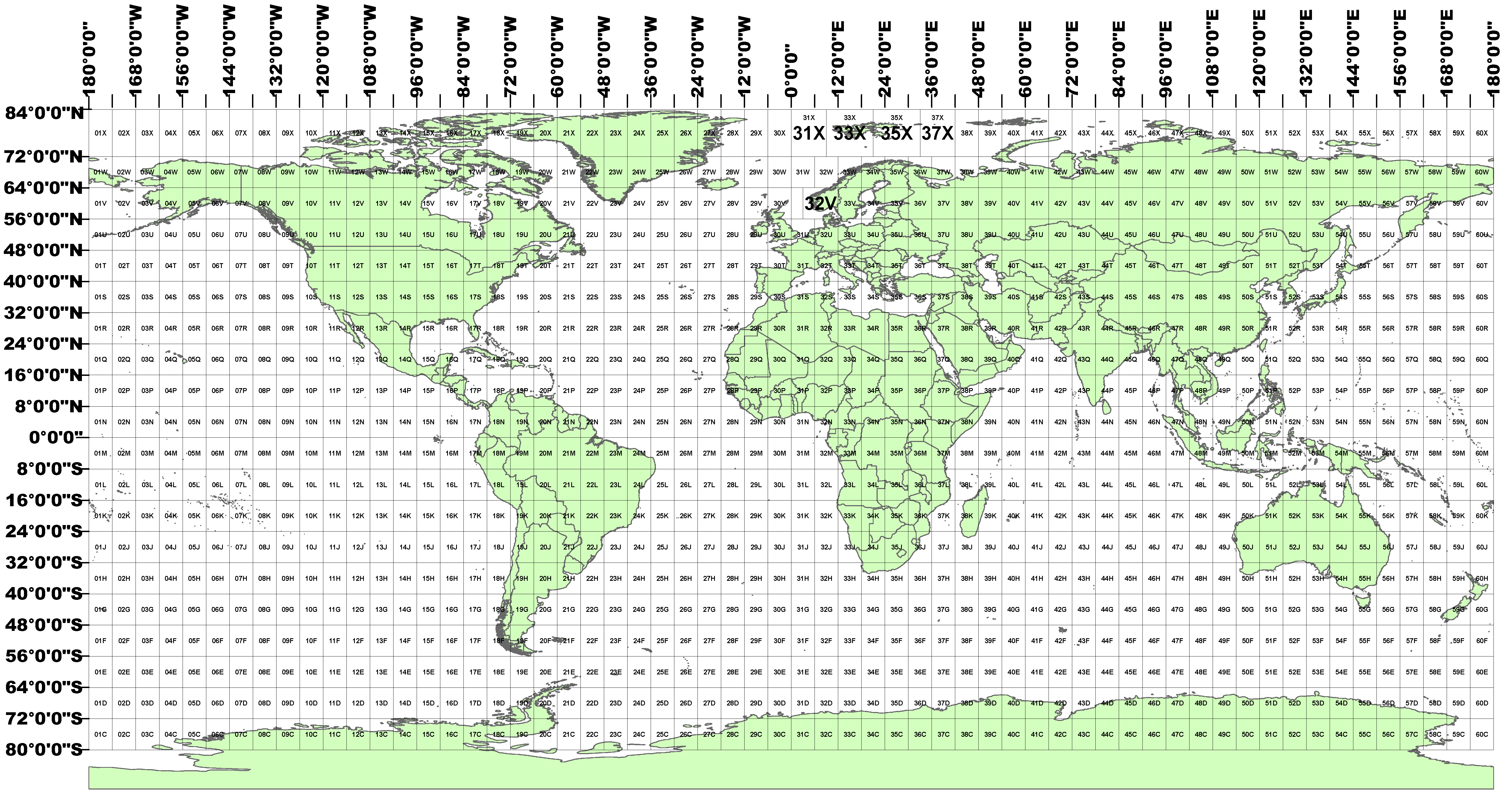
Figure 1: The Military Grid Reference System showing the 6° x 8° grid cells.
Naming Conventions
HLS L30, S30, and VI data products are distributed as Cloud Optimized GeoTIFF (COG) files and follow a consistent naming convention. (Note: OPERA-DIST and OPERA-DSWx products follow their own distinct naming conventions; please refer to their respective User Guides for details).
Data is organized and distributed as granules, which represent a distinct satellite observation tied to a geographic area (tile) and acquisition datetime. The granule ID identifies this unique acquisition and serves as both the name of the directory containing all individual layers, and the basename of the layer files themselves:
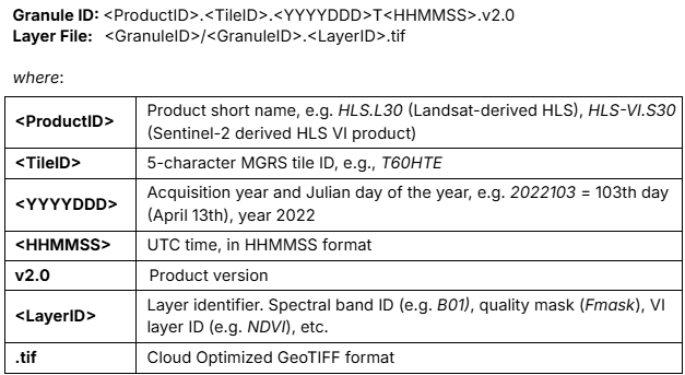
Depending on the download platform used, a granule directory may also contain additional files, including a CMR metadata file (*.cmr.xml), file size and checksum values (*.json), and a true-color browser image (*.jpg).
Spectral Bands
Input data products for HLS processing include Landsat 8/9 (Level-1TP, collection 2) OLI top-of-atmosphere reflectance or TIRS top-of-atmosphere brightness temperature and Sentinel-2 (Level-1C) MSI top-of-atmosphere reflectance (Figure 2). A series of radiometric and geometric corrections are applied to convert data to surface reflectance, adjust for BRDF differences, and spectral bandpass differences. All Landsat-8/9 OLI and Sentinel-2 MSI reflective spectral bands nomenclatures are retained in the HLS products (Table 1).
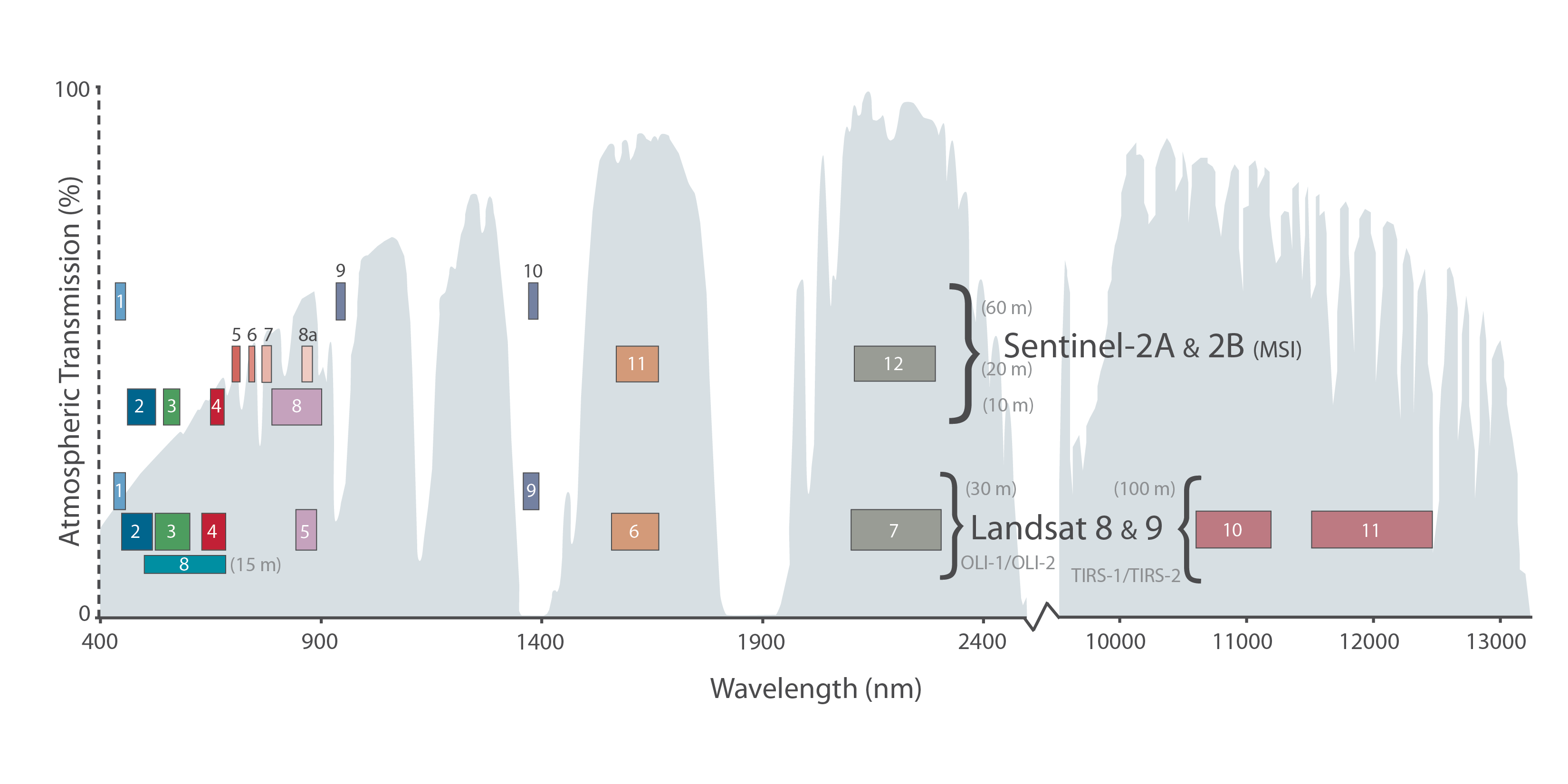
Figure 2: Graph generated by the Band Comparison Tool showing the location of bands on the electromagnetic spectrum for each HLS source instrument. The atmospheric transmission values for this graphic were calculated using MODTRAN for a summertime mid-latitude hazy atmosphere (circa 5 km visibility).
Table 1: Spectral bands for the v2.0 HLS L30 and S30 products with their corresponding source bands and wavelengths.
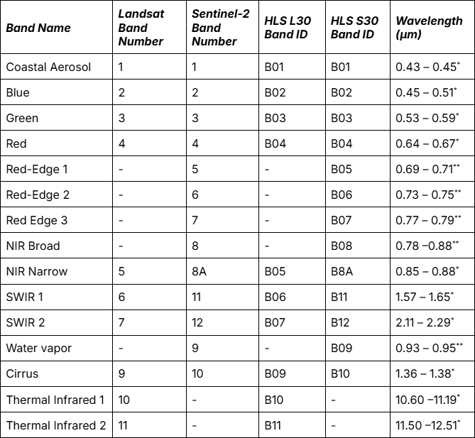
* from OLI specifications
** from MSI specifications
Data Resolution and Extent
Temporal Resolution and Extent
By harmonizing data from multiple satellite sensors, HLS significantly increases the temporal resolution, or frequency, of Earth surface observations, which is critical for operational monitoring and scientific applications that require dense time series. To quantify the cloud-free observation frequency, the HLS team evaluated 2022 data globally and found that the combination of Landsat 8/9 and Sentinel-2 A/B provided a global average median revisit interval of ~1.6 days, and a median revisit of ~2.2 days on average in data-scarce tropical regions. To determine the “global average median revisit interval,” the median time between cloud-free satellite overpasses for every individual pixel was calculated and then averaged globally (Zhou et al., 2025). A recent re-analysis with 2025 HLS data, which includes the newly operational Sentinel-2C satellite, found that this global average median revisit interval was further improved to ~1.4 days globally and ~1.9 days in the tropics (Figure 3). However, due to seasonal trends in cloud cover and high-latitude solar elevation, there can be significant variability in the number of clear observations each month, as seen in the Figure 4 animation.
The temporal coverage of the HLS v2.0 dataset begins with Landsat 8 data in 2013 and extends to the present, and includes data from Landsat 9 from 2021 and Sentinel-2 A/B/C from 2015, 2017 and 2024, respectively. The dataset is generated continuously in an analysis ready data format (ARD) and currently has a latency (time from acquisition to availability) typically 2 – 3 days, depending on ancillary data availability. However, the HLS low latency (HLS-LL) product is currently underway, which will greatly reduce this delay to better support time-sensitive monitoring and applications.

Figure 3: The median revisit interval (in days) of HLS for 2025 (top) and 2022 (bottom).
Figure 4: The total number of clear HLS observations for each month in 2025 (top) and 2022 (bottom).
Spatial Resolution and Extent
The current HLS v2.0 primary data products are provided at a 30 meter spatial resolution due to the harmonization process where the native 10 meter and 20 meter Sentinel-2 spectral bands are spatially co-registered and resampled to match the 30 meter Landsat data. However, a 10 meter HLS solution was recently selected during the latest Satellite Needs Working Group (SNWG) assessment cycle, laying the groundwork for an even higher-resolution harmonized product suite in future releases.
Spatially, HLS v2.0 covers all the global land area except Antarctica, as depicted in the land mask (Figure 5) derived from the NOAA shoreline dataset. Antarctica is excluded because of low solar elevations which compromise the plane-parallel atmospheric correction. Polar regions located at latitudes >82° are beyond the northern reach of the sensors, and image acquisition does not occur in the high latitudes during winter when the sun is too low on the horizon. Also note that Landsat or Sentinel-2 sensors may not acquire regularly over some small islands.
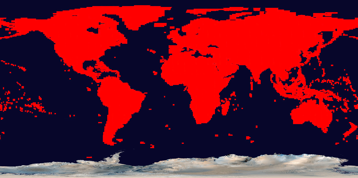
Figure 5: HLS V2.0 provides near global coverage, including major islands but excluding Antarctica.
Primary Data Products
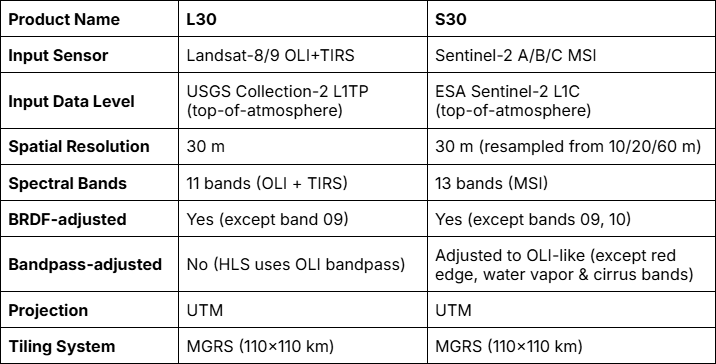
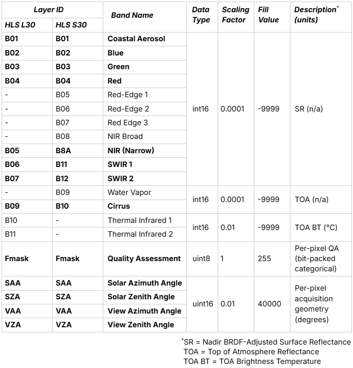
The primary HLS products, L30 and S30, form the core surface reflectance datasets of the HLS product suite. Through view angle normalization and spectral bandpass adjustments, Landsat 8/9 and Sentinel-2 imagery are harmonized into a seamless 30-meter dataset (Table 2). Delivered as Cloud Optimized GeoTIFFs (COGs), each product includes the core spectral bands alongside supplementary layers, including sun and view angles and a Quality Assurance layer (Fmask) to flag clouds, shadows, and aerosols (Table 3).
Quality Assurance Layer (Fmask)
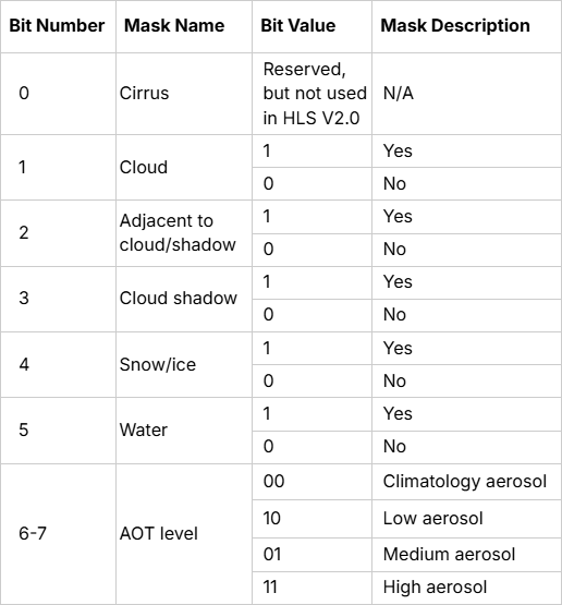
The primary HLS (L30 and S30) and HLS-VI data products are all delivered with a per-pixel Quality Assessment (QA) layer derived from the Fmask and atmospheric correction algorithms. When working with this QA band, users should pay special attention to how the data is aggregated into the final 30-meter product. Because native Landsat and Sentinel-2 inputs must be resampled to fit a common grid, the resulting QA values are a composite of their underlying sub-pixels. If any overlapping inner pixel contains a specific QA label (such as water, snow, or the 150m “adjacent to cloud” buffer), that corresponding bit is activated in the final 30m output pixel. For aerosol levels, the highest level present in the sub-pixels is retained. As a result of this process, the QA bits are not mutually exclusive, and a single pixel may simultaneously flag multiple conditions. The Fmask layer is delivered as an 8-bit bit-packed integer (Table 4); users unfamiliar with bitwise operations should consult Appendix A in the official HLS v2.0 User Guide for a straightforward tutorial on decoding these flags using simple integer arithmetic.
Table 4: Description of the bits in the QA layer. Bits are listed from the least significant bit (bit 0) to the most significant bit (bit 7). The two bits on aerosol optical thickness (AOT) level, bits 6 and 7, form a single unit – for example, 01 means 0 for bit 6 and 1 for bit 7, representing medium AOT.
Metadata
The primary HLS (L30 and S30) and HLS-VI data products are delivered with metadata embedded in their COG files and, depending on the downloading platform used, a per-granule external Common Metadata Repository (CMR) .xml file. This metadata contains valuable information, including global attributes and dataset specific attributes pertaining to the granule. For more information on the metadata attributes, please refer to the HLS v2.0 User Guide.
Table 2. HLS primary surface reflectance products specifications.
L30
The HLS L30 product provides surface reflectance and brightness temperature data derived from Landsat 8 and 9 (OLI/TIRS) Level-1TP inputs and is delivered as band-separated Cloud Optimized GeoTIFFs (COGs). The data undergoes a standardized processing pipeline that includes atmospheric correction, Fmask-based cloud masking, spatial co-registration to the Sentinel-2 tiling grid, and BRDF normalization. For a comprehensive technical breakdown of these steps, please refer to the Algorithms section.
S30
The HLS S30 product provides surface reflectance data derived from Sentinel-2A/B/C (MSI) Level-1C inputs and is delivered as band-separated COGs. To ensure true harmonization with the L30 product, the data undergoes following processing pipeline: atmospheric correction, Fmask-based cloud masking, spatial co-registration to L30 resolution, BRDF normalization, and bandpass adjustment. For a comprehensive technical breakdown, please refer to Algorithms.
Table 3. The layers delivered with the HLS L30 and S30 products. Band names in bold denote common layers present in both the L30 and S30 products.
HLS-LL
The HLS low-latency (HLS-LL) products will extend the harmonized L30 and S30 surface reflectance data to near-real-time delivery, reducing the current latency of two to three days to a target latency of six hours or less. This accelerated delivery is designed to meet high-priority science needs and support critical, time-sensitive applications such as rapid disaster response, active wildfire tracking, agricultural monitoring, and early drought detection.
Developed as an SNWG Cycle 4 solution, HLS-LL is currently in the implementation phase and will be forward-processed from Landsat 8/9 and Sentinel-2 A/B/C imagery, with initial data delivery expected in early 2027. Evaluations to determine whether HLS-LL can replace the core data products, strictly adhering to the same harmonization standards, are ongoing.
Users can track the progress of the product availability and technical details here.
Secondary Data Products
HLS secondary products currently consist of the vegetation indices product (HLS-VI) produced by the HLS team and the Land Surface Disturbance (OPERA-DIST) and Dynamic Surface Water extent (OPERA-DSWx) data products from the OPERA project at the NASA Jet Propulsion Laboratory. These data products are derived from HLS L30 and S30 surface reflectance and, along with HLS-LL, maintain the same spatial resolution/extent, map projection, and temporal resolution/extent as the primary products.
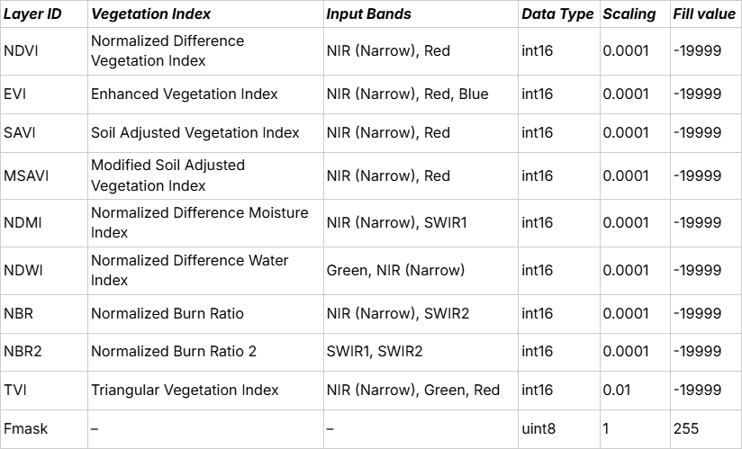
HLS-VI
The HLS-VI product currently includes nine Vegetation Indices (VI) layers derived from different combinations of the spectral bands (Table 5). These indices serve as a valuable resource for monitoring vegetation dynamics, such as crop growth, forest loss, and disturbance severity and recovery. Generated directly from the corresponding HLS L30 and S30 products, these datasets are provided as band-separated COGs and seamlessly utilize the same MGRS tiling system and naming conventions as the primary products. Like the primary products, HLS-VI granules are also delivered alongside a QA layer (Fmask) and contain metadata attributes specific to the HLS-VI product (listed in the HLS VI User Guide).

The Harmonized Landsat Sentinel-2 Project Releases Vegetation Indices
These new vegetation indices offer the same near-global coverage, and 30-meter spatial resolution as the initial HLS products.
Table 5: The VI layers delivered with the HLS-VI product and their bands used for computation. All layers are provided for both L30 and S30 derived HLS-VI products.
VI Descriptions and Equations
Normalized Difference Vegetation Index
The Normalized Difference Vegetation Index (NDVI) serves as a ubiquitous tool in remote sensing, offering insights into vegetation presence and vitality. By combining near-infrared (NIR) and red reflectance, NDVI provides indications of vegetation density and stress levels, proving invaluable for environmental monitoring and vegetation assessment (Tucker 1979).
L30 equation:

S30 equation:

Enhanced Vegetation Index
The Enhanced Vegetation Index (EVI) was developed to mitigate atmospheric influences and increase sensitivity to high biomass (Huete et al., 1997; Huete et al., 2002). EVI is particularly useful in regions with dense vegetation cover or significant atmospheric interference.
L30 equation:

S30 equation:

Soil Adjusted Vegetation Index
In regions with high soil reflectance, the Soil Adjusted Vegetation Index (SAVI) diminishes soil brightness effects on vegetation detection (Huete 1988). By introducing a soil adjustment factor, SAVI enhances vegetation detection sensitivity, especially in arid and semi-arid areas where soil reflectance can compromise index accuracy.
L30 equation:

S30 equation:

Modified Soil Adjusted Vegetation Index
An adaptation of SAVI, the Modified Soil Adjusted Vegetation Index (MSAVI) further improves vegetation detection accuracy, particularly in areas with dense vegetation or high soil reflectance (Qi et al. 1994). By addressing soil brightness and saturation effects from abundant vegetation cover, MSAVI emerges as a reliable indicator of vegetation health across various ecosystems.
L30 equation:

S30 equation:

Normalized Difference Moisture Index
Developed to quantify vegetation moisture content or water stress, the Normalized Difference Moisture Index (NDMI) leverages the difference between NIR and shortwave infrared (SWIR) reflectance (Wilson and Sader, 2002). NDMI’s ability to discern moisture content makes it instrumental in monitoring vegetation health and water availability.
L30 equation:

S30 equation:

Normalized Difference Water Index
The Normalized Difference Water Index (NDWI) is a remote sensing index used to detect the presence and changes in water bodies within an image (McFeeters, 1996). It measures the difference in NIR and green band reflectance. High NDWI values indicate the presence of water, while low values indicate non-water features like soil or vegetation. NDWI is particularly useful for monitoring changes in surface water bodies, such as lakes, rivers, and wetlands, and for assessing water-related environmental dynamics.
L30 equation:

S30 equation:

Normalized Burn Ratio
The Normalized Band Ratio (NBR) is used to assess vegetation health and monitor disturbances such as wildfires (Key and Benson, 2006). It is calculated as the normalized difference between the NIR and SWIR1 bands. Positive NBR values typically indicate healthy vegetation, while negative values suggest burned or stressed vegetation. NBR is valuable for assessing changes in vegetation conditions, particularly in areas affected by fire, drought, or other environmental disturbances.
L30 equation:

S30 equation:

Normalized Burn Ratio 2
Developed for assessing wildfire burn severity, the Normalized Burn Ratio 2 (NBR2) measures the disparity between SWIR1 and SWIR2 reflectance. By offering assessments of vegetation health and burn severity, NBR2 provides gradations of damage severity, aiding in wildfire impact assessments.
L30 equation:

S30 equation:

Triangular Vegetation Index
The Triangular Vegetation Index (TVI) is a vegetation index derived from remote sensing data, particularly from multispectral imagery (Broge and Leblanc, 2001). It is calculated using the red, green, and NIR bands to estimate vegetation health and vigor. TVI enhances the contrast between vegetation and soil, making it useful for monitoring changes in plant biomass and stress levels. It’s particularly effective in assessing vegetation health in agricultural fields and natural ecosystems.
L30 equation:

S30 equation:

OPERA-HLS
Established by the Jet Propulsion Laboratory in response to the Satellite Needs Working Group (SNWG), the OPERA project develops specialized near-global data products to meet the high-priority needs of federal agencies. Within this initiative, the OPERA-HLS suite leverages HLS data to generate highly responsive environmental monitoring datasets. Specifically, this HLS imagery serves as the primary foundational input for two distinct products: OPERA-DIST (Land Surface Disturbance) and OPERA-DSWx (Dynamic Surface Water eXtent).
OPERA-DIST
The OPERA-DIST product suite maps per-pixel vegetation cover loss and generic land surface disturbance trends. Because it utilizes the HLS surface reflectance data as its primary input, it is able to detect these environmental changes at a highly responsive rate. The suite is offered as two distinct products: DIST-ALERT, which provides land mass disturbance alerts released at the same cadence as the source HLS imagery; and DIST-ANN, which provides an annual summary of confirmed disturbance changes from the previous year. The DIST products are distributed as Cloud-Optimized GeoTIFFs (COGs) and are publicly accessible through the Land Processes Distributed Active Archive Center (LP DAAC).
OPERA-DSWx
The OPERA-DSWx product suite maps pixel-wise spatial and temporal variations of surface water inundation across all near-global landmasses (excluding Antarctica). The optical DSWx product relies on the primary HLS datasets to detect water features, supplemented by three ancillary inputs to improve accuracy: the Copernicus Global Land Cover discrete classification map, the ESA WorldCover map, and a global Digital Elevation Model (DEM). OPERA-DSWx is distributed as COGs and are accessible through NASA’s Physical Oceanography Distributed Active Archive Center (PO.DAAC).
HLS Product Evaluation
To evaluate HLS product consistency, the HLS team analyzed over 136 million cloud-free samples from same-day L30/S30 observation pairs, collected during 2021–2022 across 96 globally distributed tiles. Our analysis revealed distinct performance patterns across different spectral bands.
For the red, near-infrared (NIR), and two shortwave infrared (SWIR) bands, the surface reflectance differences between sensors remained below 4% of the mean Landsat surface reflectance values—all significantly smaller than the corresponding differences in top-of-atmosphere (TOA) data. These results confirm the collective effectiveness of the harmonization process for these spectral regions.
However, the two blue bands and a green band—which are highly sensitive to aerosol contamination—showed a different pattern. In these bands, the between-sensor surface reflectance differences were actually greater than those observed in the TOA data, primarily due to noise introduced during atmospheric correction processing.
Despite this limitation in the blue and green bands, surface reflectance data remains more scientifically valuable than TOA reflectance. This is because surface reflectance products are largely free from the volatile temporal variations caused by changing atmospheric conditions, making them more directly related to terrestrial biological and physical processes (Ju et al., 2025).We further assessed the consistency of HLS VI products using the same image pairs, finding strong overall agreement between sensors. Discrepancies primarily increased under specific conditions, such as low winter solar angles, terrain shadows, and high aerosol loads, with extreme vegetation values also introducing noticeable uncertainties. To help users manage these factors, we provide standard deviations of discrepancies stratified by both aerosol levels and VI values. These metrics enable researchers to effectively account for VI uncertainties within their specific applications and encourage the consideration of VI-specific value ranges during analysis (Zhou et al., 2026).